Managing materials

In this section we describe how to create and assign the resin (fluid) and porous materials in Lizzy. All operations can be performed using the LizzyModel user-facing methods.

Defining the resin

The resin represents the fluid that will fill the part. It is defined by its dynamic viscosity and must be created and assigned before initialising the solver.

To create a resin, use the create_resin() method, providing a unique name and a dynamic viscosity value [Pa·s]:

model.create_resin("resin", viscosity=0.1)

A Resin object is created and stored in the model. To assign it to the simulation, use the assign_resin() method:

model.assign_resin("resin")

Note

Only one resin can be assigned at a time. The resin must be assigned before calling initialise_solver(), otherwise an error will be raised.

Porous materials in Lizzy

In Lizzy, a porous material is represented by the PorousMaterial class. This class encapsulates the properties of a porous material, including its permeability, porosity, and thickness. Each material is defined by the following properties:

Name: A unique string identifier for the material.
Permeability (k1, k2, k3): The permeability of the material in three principal directions (in m²).
Porosity: The porosity of the material (dimensionless, between 0 and 1).
Thickness: The thickness of the material (in m). A material can represent a single layer of fabric, or a multi-layer laminate. In the latter case, the thickness represents the total thickness of the laminate.

The current version of Lizzy does not allow to compose a multi-layer laminate automatically by defining its layers. Instead, the user must compute the equivalent permeability, porosity, and thickness of the laminate externally and define a single PorousMaterial object representing the entire laminate. This is typically done using arithmetic average schemes [2] [3]. We plan to implement an automated multi-layer laminate definition feature in future releases.

Creating materials

Note

The following operations are to be performed before the solver is initialised by calling initialise_solver().

We can create a porous material using the create_material() method. This method requires a unique name for the material, the permeability values (as a tuple), porosity and thickness. For example, to create a material named “material_01” with permeability values of 1E-10 m² in all directions, a porosity of 0.5 and a thickness of 1.0 mm, we would type:

model.create_material("material_01", (1E-10, 1E-10, 1E-10), 0.5, 0.001)

A PorousMaterial object is created and stored in the model, but it is not assigned yet.

Creating an orientation Rosette

When working with anisotropic materials, it is necessary to define how the principal directions of permeability are oriented in the domain. To do so, we can create a Rosette object. A rosette is a local basis \(\hat e_1, \hat e_2, \hat e_3\) that defines an orientation in space. When associated to a material, the principal directions of permeability will be aligned with the basis defined by the rosette. In Lizzy, we don’t define the basis components directly. Instead, for any given rosette, we define a single orientation vector \(u_1\) that will be projected onto the mesh elements to calculate the local basis \(\hat e_1, \hat e_2, \hat e_3\) (more on this below). To create a rosette, we can use the create_rosette() method by providing a name for the rosette and the vector \(u_1\). For example, we can create a rosette named “rosette_01” with a vector \(u_1\) oriented along (1, 1, 0) by typing:

model.create_rosette("rosette_01", (1,1,0))

Assigning materials

To assign a material to a labeled domain, we use the assign_material() method, providing the following arguments:

the name of the material to assign
the name of the mesh domain where we want to assign it
the rosette of orientation

For example, to assign the material “material_01” to a mesh domain labelled as “domain_01” and orient it using using the rosette “rosette_01”, we would type:

model.assign_material("material_01", "domain_01", "rosette_01")

When the assignment happens, the remaining components of the local rosette (\(\hat e_1, \hat e_2, \hat e_3\)) are calculated and registered for as follows:

\(\hat e_1\): is calculated as the projection of \(u_1\) along the normals of the elements in the domain
\(\hat e_3\): is calculated as the normal of the elements in the domain
\(\hat e_2\): is calculated as \(\hat e_1 \times \hat e_3\)

Note

If a rosette is not provided, a default orientation is used with \(\hat e_1, \hat e_2, \hat e_3\) aligned with global axes \(e_1, e_2, e_3\). This can be convenient when working with isotropic materials, since we don’t care about their orientation. For example:

k_iso = 1.0E-11
model.create_material("material_iso", (k_iso, k_iso, k_iso), 0.5, 1.0)
model.assign_material("material_iso", "domain_01")

Element-wise manipulation

After assigning a material to a domain, the material properties are stored as attributes directly on each element object. This allows to overwrite individual element properties with arbitrary spatial distributions that are not expressible through the standard assign_material() workflow.

Two methods are available for this:

get_elements(): returns the list of all elements in the mesh.
get_element_by_idx(): returns a single element by its integer index.

The editable element attributes are:

elem.h: thickness (float, in m).
elem.porosity: porosity (float, dimensionless).
elem.k: permeability tensor (3×3 numpy array, in m²).

Example: spatially varying thickness

Say we have a part of length \(L\) and want to assign a linearly varying thickness \(h(x)\), going from \(h(0) = 1\) mm to \(h(L) = 5\) mm. We first assign a material (which sets a uniform thickness), then overwrite the thickness element by element:

import numpy as np

# assign material to the domain (sets a uniform thickness initially)
model.assign_material("material_01", "domain")

# iterate over all elements and overwrite the thickness
L = 1.0  # part length in m
for elem in model.get_elements():
    x = elem.centroid[0]
    elem.h = 0.001 + 0.004 * (x / L)

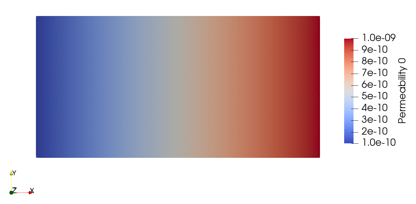
Example: spatially varying permeability

The same approach applies to permeability. The elem.k attribute stores the full 3×3 permeability tensor in the global frame. For an isotropic permeability that varies linearly along x, we can write:

import numpy as np

model.assign_material("material_01", "domain")

L = 1.0
for elem in model.get_elements():
    x = elem.centroid[0]
    k_val = 1e-10 + 9e-10 * (x / L)  # varies from 1E-10 to 1E-9 m²
    elem.k = np.diag([k_val, k_val, k_val])

Note

Element-wise manipulation must be performed before calling initialise_solver(). Modifying element properties after solver initialisation is not supported, as it would imply non-trivial physical implications during an ongoing filling (e.g. changing the thickness of an already-filled element).