Channel Flow
This case demonstrates a minimal implementation of the solver. We will use Lizzy to simulate the filling of an isotropic rectangular panel, prescribing a one-dimensional flow. This classical infusion scenario is known as the Channel Flow experiment [1].
All files used in this tutorial are available in the tutorials/channel_flow folder. We recommend you download the mesh alone and create the script yourself following the tutorial.
Preparing the working folder
Create a new folder in a preferred location and name it something descriptive of the infusion scenarion, like channel_flow or similar. We will refer to this folder as the working folder and the entire Lizzy workflow will be run inside here. Copy the mesh file into the working folder. Create a new python script in the working folder. This will be the only python script we will need. In this example, the file is named channel_flow.py, but any name will do.
The mesh
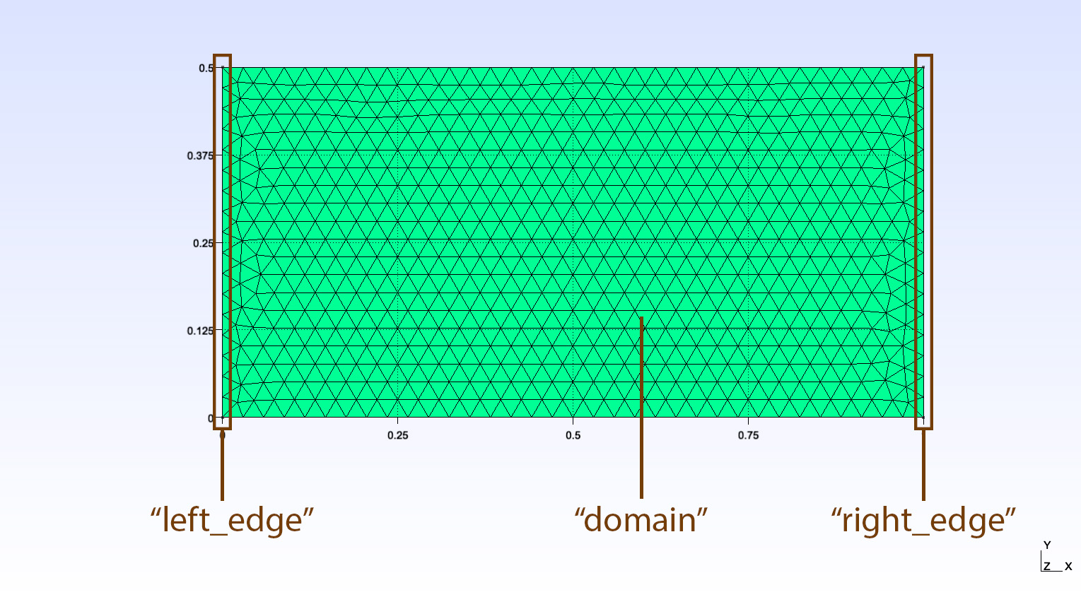
The mesh represents a rectangular domain 1 m wide and 0.5 m tall. The mesh contains 3 domain tags (“physical groups” in msh format):
left_edge: line tag assigned to the left edge of the mesh
right_edge: line tag assigned to the right edge of the mesh
domain: elements tag assigned to all elements in the mesh
These tags will be used to identify regions of the mesh for assignment of material properties and boundary conditions.
Importing Lizzy
In the first line of the script, let’s import Lizzy by:
import lizzy as liz
Setting up logging
Lizzy uses the standard Python logging module to log messages. By default, nothing will output to console (as recommended practice when using the logging moule). To get some information at runtime, let’s set up the logger to the INFO level:
import logging
logging.basicConfig(level=logging.INFO)
Creating the Lizzy model
Every simulation model in Lizzy is defined using the LizzyModel class. This is the main class of the solver and provides all APIs necessary to fully define a simulation scenario.
The first expression in any Lizzy script is to create the LizzyModel that will be used in the simulation:
model = liz.LizzyModel()
From now on, we will use this LizzyModel object to access all the relevant APIs.
Reading the mesh file
Let’s read the mesh file that we have copied:
model.read_mesh_file("ChannelFlow.msh")
Make sure that the path given points to the mesh file that we have copied in the folder. In this example, both the script and the mesh are in the working folder. If your folder structure is different, adjust the mesh path accordingly.
Setting simulation parameters
Now that the mesh is read, we need to define a few settings. We can do so using the set_simulation_parameters() method. We will set the to write a solution state every 10 seconds in the results file, and we will activate a progress bar that will show us solution progress at runtime:
model.set_simulation_parameters(output_interval=30, progress_bar=True)
Note
There is no particular order in the script as where the set_simulation_parameters() method should be called, as long as it is done before the solver is initialised by the initialise_solver() method (further on). Failure to do so, or omitting the call entirely, will result in running the simulation with default values.
Creating materials
Next, define the resin (fluid) to be used in the simulation:
model.create_resin("resin", viscosity=0.1)
model.assign_resin("resin")
The create_resin() method takes a name and a dynamic viscosity value [Pa.s]. The resin must be assigned to the model using assign_resin().
Now we can define the properties of the material in the mesh and assign it to a mesh domain:
model.create_material("test_material", (1E-10, 1E-10, 1E-10), 0.5, 0.005)
model.assign_material("test_material", 'domain')
The method create_material() instantiates a PorousMaterial object which is stored in the model. The arguments of create_material() are:
name(str): the name assigned to the material, used to identify it for later assignment.k_vals(tuple[float, float, float]): permeability values \((k_1, k_2, k_3)\) in principal directions [m²].porosity(float): the fraction of total material volume not occupied by solid material (1 - Vf).thickness(float): the thickness of the material in the out-of-plane direction [m].
Note that no material orientation was defined. This is ok because the material declared is isotropic. Behind the scenes, Lizzy assigns a default rosette aligned with the global x, y, z axes. Local material orientations and zone-specific rosettes will be detailed in more advanced examples.
Note
Each material tag present in the mesh must be assigned a material, otherwise initialisation will raise an error.
Boundary conditions
Next, we will create some boundary conditions. In this example we will create a pressure inlet on the left edge of the mesh. Inlets are created with a name and a pressure value, then assigned to a mesh boundary:
model.create_pressure_inlet("inlet_left", 1E+05)
model.assign_inlet("inlet_left", "left_edge")
The create_pressure_inlet() method takes the inlet name and the prescribed pressure value [Pa].
We can also create a vent gate where perfect vacuum is prescribed (p=0 Pa) on the right edge of the mesh:
model.create_vent("vent_right", 0.0)
model.assign_vent("vent_right", "right_edge")
Creating a vent is not strictly necessary (if no vent is defined, the solver will automatically assign a pressure p=0 Pa to all unfilled nodes), but doing so we can prescribe a different vacuum pressure to be used.
Initialise solver
Once the simulation model has been completely defined, we must call the initialise_solver() method to finalise the model. It is useful to think of this as the expression that finalises the model setup phase. Therefore this method should be called last, after all assignments have been made (inlets, materials, sensors, controls, etc…):
model.initialise_solver()
Solve
Our model is now ready for solving. The next step is to call the solve() method to run the filling simulation:
model.solve()
The solve() method returns a Solution object, which can be captured optionally. The same can also be fetched from the model latest_solution attribute, so there is usually no need to capture the returned object.
Write results
The next logical step after solving is to indicate to Lizzy that we want to write the results to file.
The write-out of results in Paraview-compatible format is handled by the save_results() method:
model.save_results()
The save_results() method several optional arguments (see API reference). If we call it with no arguments, then a default results folder and file name will be created.
The full script
import lizzy

import logging
logging.basicConfig(level=logging.INFO)

model = lizzy.LizzyModel()
model.read_mesh_file("ChannelFlow.msh")
model.set_simulation_parameters(output_interval=30, progress_bar=True)

model.create_resin("resin_01", 0.1)
model.assign_resin("resin_01")

model.create_material("domain_material", (1E-10, 1E-10, 1E-10), 0.5, 0.005)
model.assign_material("domain_material", 'domain')

model.create_pressure_inlet("inlet_left", 100000)
model.assign_inlet("inlet_left", "left_edge")

model.create_vent("vent_right", 0.0)
model.assign_vent("vent_right", "right_edge")

model.initialise_solver()
model.solve()

model.save_results()
Running the script
To run the script, open a terminal and navigate to the working folder. Make sure that the Python environment where Lizzy is installed is activated, then simply run the script we have just created.
Since both logging and progress bar are activated in this example, on the console you will read some runtime output like this:
|    _)
|     | _  / _  /  |  |
____| _| ___| ___| \_, |
                ___/
        v0.1.0

INFO:lizzy.io: Reading mesh file: ChannelFlow.msh
INFO:lizzy.mesh: Creating Mesh with 3422 elements and 1800 nodes...
INFO:lizzy.solver: Preprocessing...
INFO:lizzy.solver: Solving started on 3422 elements and 1800 nodes
Fill progress: 100%|██████████████████████████████████| t=2499.89s [00:00<00:00]
INFO:lizzy.solver: Solve completed in 0.41 seconds
INFO:lizzy.solver: Empty CVs: 0, fill time: 2499.89 seconds
INFO:lizzy.io: Saving results...
INFO:lizzy.io: Results saved in results/ChannelFlow_RES
Congratulations, you have just run your first Lizzy simulation!
Solution visualisation
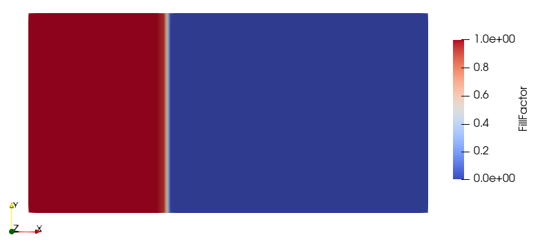
The results are saved in a folder results which is created in the current working directory of the interpreter. By default, Lizzy will save results in the XDMF format, leveraging HDF5 database in binary format to store the actual data. Load the file ChannelFlow_RES.xdmf into Paraview to visualise the results in a time series: when prompted, make sure to select `Xdmf3 Reader S` to avoid formatting issues.
Lizzy will save the following fields: “FillFactor”, “FreeSurface”, “Pressure”, “Velocity”. In the picture, an example of fill factor at t=300s.